0. Terms
- Saturating non-linearities
- Intuitions:
A saturating activation function squeezes the input. - Definitions:
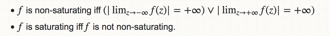
- Examples:
- Rectified Linear Unit (ReLU) activation function is non-saturating
- Sigmoid activation function is saturating
- Hyperbolic tanget function(tanh)is saturating
- Intuitions:
- Internal Covariate Shift
- the change in the distribution of network activations due to the change in network parameters during training
1. Overview
- Phenomenon: internal covariate shift
- classical NN training is slow and hard to train with saturating non-linearities
- Solution: making normalization a part of the model architecture and performing the normalization for each training mini-batch
- Advantages:
- higher learning rates(train faster)
- be less dependent on parameter initialization
- it can also replace the role of Dropout, in some cases
2. Why
2.1 Why mini-batch
- mini-batch gradient is more robust
- mini-batch calculation is more efficient due to parallelism (i.e, GPU)
2.2 Why(internal)covariate shift
Small changes to the network parameters amplify as the network becomes deeper(forward feeding)
When ‘the input distribution to a learning system’ changes, it is said to experience covariate shift(Shimodaira, 2000)
Consider such a network computing:
$$
l = F_2(F_1(u, \Theta_1), \Theta_2)
$$
the former output serves as the input of the latter network, and it’s equivalent that the output comes from other place rather than the former layer. So it is advantageous(don’t understand well)for the distribution of the input of latter layer to remain fixed over time.
- A critical point
- Saturate non-linear activation functions, such as sigmoid, will suffer gradient vanishing if the norm of input gets too big.
- This effect is amplified as the network depth increases.
- In practice, this problem is avoided by using non-saturate functions like ReLU as well as small learning rates.
- So, what if we could control the norm of the input and make its distribution more stable?
2.3 Why Batch Normalization
- We achieve such ‘control’ by introducing the new mechanism – Batch Normalization, which reduces the internal covariate shift and accelerates network training.
- It has been long known(LeCun et al., 1998b; Wiesler & Ney, 2011)that the network training converges faster if its inputs are whitened(closer to white noise). i.e., linearly transformed to have zero means and unit variances, and decorrelated.
- Furthermore, batch normalization regularizes the model and reduces the need for Dropout(Srivastava et al., 2014).
2.4 Two problems of ‘Gradient Descent + Normalization’
- Consider whitening activations at every training step, interspersed with gradient descent. The combination of update to b, a learned bias, and subsequent change through normalization will lead to no change in the output and, also, the loss function w.r.t the bias term, b. Thus, b will grow indefinitely while the loss remains ‘fixed’ w.r.t b.
- Consider a deep NN with single unit at each layer and the forward equation is $y = x\prod_{i=1}^l w_i$. After back propagation, we have $y’ = x\prod_{i=1}^l (w_i - \epsilon g_i)$. For instance, the term $\epsilon^2g_1g_2\prod_{i=3}^l w_i$ will goes to infinity if $l$ is big(deep network)and ${w_i}_{i\ge 3}$ are bigger than $1$. This will lead to update unstability and gradient vanishing for saturating non-linear activation functions.
- Main issue with the above problems: the gradient descent procedure doesn’t take into account the normalization process.
- To address this issue, one should ensure that the network always produces activations with the desired distribution. (output -> BN -> activation)
3. Methodology
3.1 Why not full whitening of each layer’s input?
- Computationally expensive
For back propagation, we need to compute the Jacobians:
$$
\frac{\partial \text{Norm}(x,\chi)}{\partial x} \text{ and }\frac{\partial \text{Norm}(x,\chi)}{\partial \chi}
$$
Ignoring the second term will lead to the first problem mentioned above. And, the second term requires the covariance matrix of the design matrix $\chi$, along with its square root matrix. However, for deep networks, the training set $\chi$ is usually quite large.
- Not everywhere differentiable
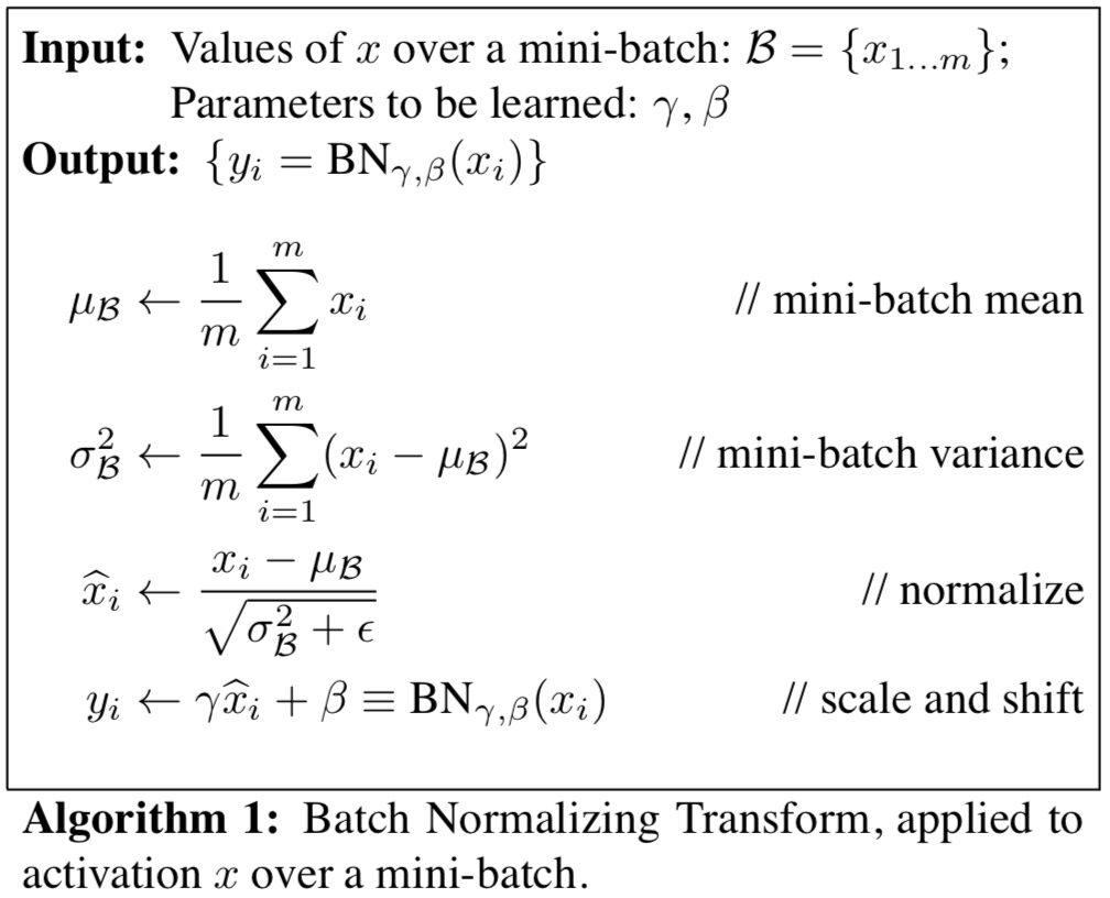
3.2 Normalization via Mini-Batch Statistics
Two simplifications:
Instead of whitening the features in layer inputs and outputs jointly, we will normalize each scalar feature independently, by making it have the mean of zero and the variance of 1
To ensure the representation power of certain layer, we introduce, for each activation $x^{(k)}$, a pair of parameters $\gamma^{(k)}, \beta^{(k)}$, which scale and shift the normalized value:
$$
y^{(k)} = \gamma^{(k)}\widehat{x}^{(k)} + \beta^{(k)}
$$The two parameters are updated through the same way as other network parameters.
Since we use mini-batches in stochastic gradient training, each mini-batch produces estimations of the mean and variance of each activation
The Batch Normalization Algorithm